Improving the GAN

In my previous post, I gave an introduction to generative adversarial networks (GANs), discussed the basic training algorithm, and implemented a basic GAN for generating handwritten digits. While this basic model works well and has been shown to produce decent images, there are many difficulties that one can encounter during training, a popular one being divergence in the model performance and vanishing gradients. In this post, I’ll discuss these issues in more detail and then introduce the Wasserstein-GAN, one of the most popular and successful improvements to the standard GAN.

Flashback time…

Recapping GANs briefly, these are models which aim to generate realistic data. It is composed of two neural networks: a generator network that inputs Gaussian noise and outputs a synthetic image. The second is a discriminator network that inputs the generated image and a real image from the original dataset, from which it determines whether they are real or fake. This is analogous to a counterfeiter and a security guard in the bank. The counterfeiter’s job is to create fake dollar bills that look like real ones while the security’s job is to look at the fake money and tell whether it looks real or fake. By knowing how authentic or rubbish the fake dollar bill looks, the counterfeiter will be able to improve his quality over time.

Improving GAN training

Despite this simple setup, it must be stated that GAN’s are really hard to train. There are many contributing factors to this, a major one being that the discriminator tends to learn faster than the generator. Intuitively, the effect of this is that for any image the generator creates, the discriminator will always label it as a fake and this will eventually provide very minimal feedback or incentive for the generator to improve.

Now let’s actually dig into what this means mathematically. To understand the problem, first, let’s set aside the GAN and just think about what we are trying to achieve. Basically, we have a distribution of real data, which we can call P, and a fake data distribution called Q. Since we want to create fake data that looks like the real, we want Q’s distribution to move closer and closer to P. How do we measure this closeness between two probability distributions?

Well, one possible way to measure it is called the Kullback-Liebler Divergence or KL-divergence. This has a formula as follows:

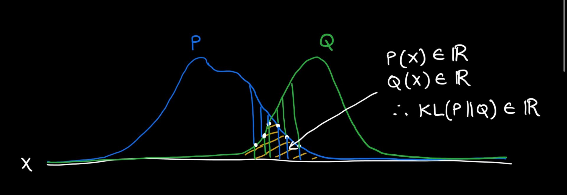
Unfortunately, there is one problem with this divergence measure – it only works if there is some small amount of overlap between the two distributions. To see this, observe the diagrams below:

In the first diagram, there is a bit of overlap between P and Q. Applying the KL formula, we will see that in this overlap region, P(x) has some real value and so does Q(x), so the KL divergence will be real-valued. But if I pull the distributions apart, as seen in the second diagram, P(x) will be real-valued in the support of x, but for those x values, the Q(x) will be 0, which means the KL divergence will blow up to infinity. This is not desirable, therefore it’s not the best choice for measuring divergence between distributions.

The next option is basically an extension of KL divergence called the Jenson-Shannon divergence (JSD). This basically finds an average of the distributions P and Q, which we can call M. It then takes the average of the KL divergence between P and M and Q and M. The equation for this is:

Now if we apply the formula for the overlapping and separated distributions, as in the two diagrams above, we’ll find that JSD will be 0 when the distributions perfectly overlap and log2 when they don’t overlap at all. So this is a step forward, we’ve got a divergence that is real-valued when the distributions are still not overlapping. Is this good enough? Nope, still not good enough!

So what’s the problem now? Well, let’s do an experiment where P is fixed and we pull Q further and further away from P like shown below:

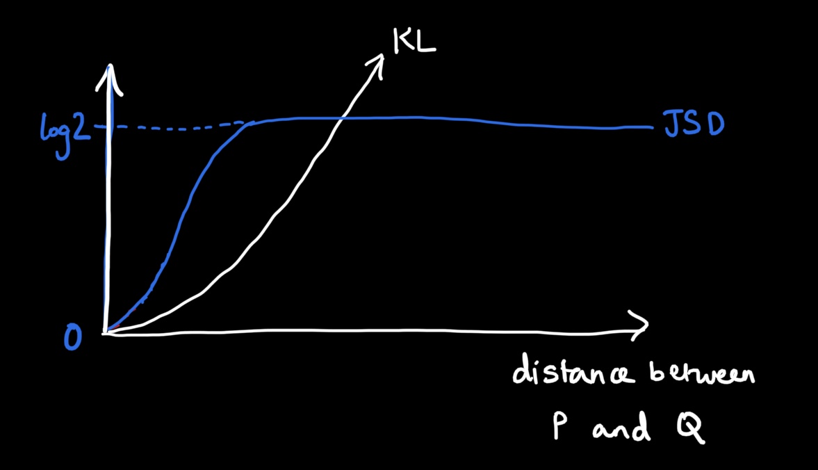
If we plot the values of the JSD, you’ll see that it starts off at 0, then slowly increases as we separate the distributions. Finally, when there is no overlap, it just plateaus at log2. For comparison, I’ve also shown the KL divergence, which just moves towards infinity as the distributions separate.

There’s a problem here: if we used the JSD for a loss function in our GAN and did the backpropagation algorithm, the gradient would be 0 when the distributions are far apart. This would lead to minimal updates in the generator’s weights, meaning no improvement in the GAN whatsoever.

This is exactly what happens with the standard minimax loss of the GAN. The authors proved in their paper that if the discriminator became optimal, then minimax loss essentially becomes a Jenson-Shannon divergence between the real and fake data distributions. So now, if the discriminator network outperforms the generator within a few iterations of training and approaches optimality, we can expect that vanishing gradients will kick in and the generator will not improve.

So then what do we do about this? What metric is effective for measuring the distance between data distributions and has a stable gradient? Enter the Wasserstein distance!

Wasserstein-GAN

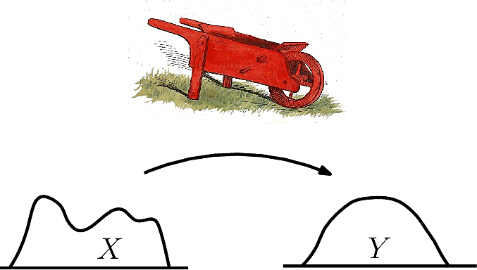
Instead of probability distributions, if we think of P and Q as piles of dirt, the Wasserstein distance basically represents the amount of effort that is required to take the pile of dirt in Q, transport it and mold it into the pile of dirt P. For this reason, it is also known as the Earth Mover’s Distance (EMD). Notice that with this metric, we are now measuring divergence in terms of the horizontal axis distance, rather than the probability densities on the vertical axis.

Wasserstein Distance represents the effort taken to shift a pile of dirt from X to create the pile of dirt in Y. Image taken from here.The equation for the Wasserstein distance is shown below.

Notice that now instead of a discriminator D that predicts the probability of an image being real, we have a “critic” C which scores an image based on how real or fake it looks. This difference is beneficial for training because the output is not bounded to 0 and 1 for real and fake; it can be any real numbered value. If the distance between distributions is large then the Wasserstein distance will be a large positive number and if small, it will be near 0. This means that gradients will also have non-zero values, which can improve training stability.

There is a catch though: one requirement for this loss function to be valid is that it must have a property called 1-Lipschitz continuity. This is just a fancy way of saying that the magnitude of the gradients must be at most 1. This mathematical requirement ensures that the loss is continuous and differentiable, but also maintains stability during training. How does one enforce this requirement? Well, two popular methods are gradient clipping and gradient penalty. Gradient clipping is where the weights are truncated to be no greater than 1. The more popular method, gradient penalty, is similar to L2 regularization in a neural network where an extra term is added to the loss function, penalizing the weights to be as small as possible.

What’s coming up next?

In summary, you now understand one of the most important issues with GAN training and how the Wasserstein-GAN addresses this. Of course, there are many other approaches that have been proposed to make training stable, an interesting one being Relativistic GANs. This essentially proposes that instead of making the discriminator compute the loss of the real and fake data separately, it would be better to use a relativistic discriminator that measures the relative realism between fakes and generated data.

In my upcoming posts, I hope to delve into some of the fun and really popular state-of-the-art GANs designed for image generation tasks. Also, being passionate about GANs for medical imaging, I hope to delve into some of the applications. Stay tuned!